portfolio tracker
- Overview
- Sheet Breakdown
Net Worth · Monthly Tracker · Markets · Cash · Metals · Retirement · Insurance - Technical Logic
Formulas · Named Ranges · The Helper Sheet - How to use
- Glossary
Overview
There are a thousand different apps on the internet to track our savings and portfolios, with each offering a particular feature that others lack. Very few apps allow us to track everything we need in a systematic way. I have found manual tracking to be the only reliable method to get a true picture of my net worth. For this reason, I set out to build a Google Sheets file to do exactly that.
With this file, the user can track their Equity, Debt, Commodities and Retirement/Insurance information.
You just need to click on following link and click on “Make A Copy”.
Potfolio Tracker Template Google Sheet
It might display “Warning: Some formulas are trying to send and receive data from external parties.” in the beginning. This is to track Gold Prices from external sources. You will need to click on Allow Access
While I have added warnings throughout the post requesting not to edit certain cells in the sheets, please feel free to experiment and create your own system which works specifically for you.
Jump to the How to use section to immediately start tracking.
Sheet Breakdown
| Name | What it tracks |
|---|---|
| Helper | Contains USDINR, Metals rates and dynamic table for charts. (Should not be edited) |
| Net Worth | Shows an overview of all assets (Should not be edited) |
| Monthly Tracker | Total of all individual assets |
| Markets | Individual Stocks/Equity Funds/Debt Funds across India and US |
| Cash | Cash/BankBalance/FD |
| Metals | SGB/Gold/Silver/Platinum |
| Retirement | PPF/EPF/NPS |
| Insurance | Term/Health/Accidental Insurance |
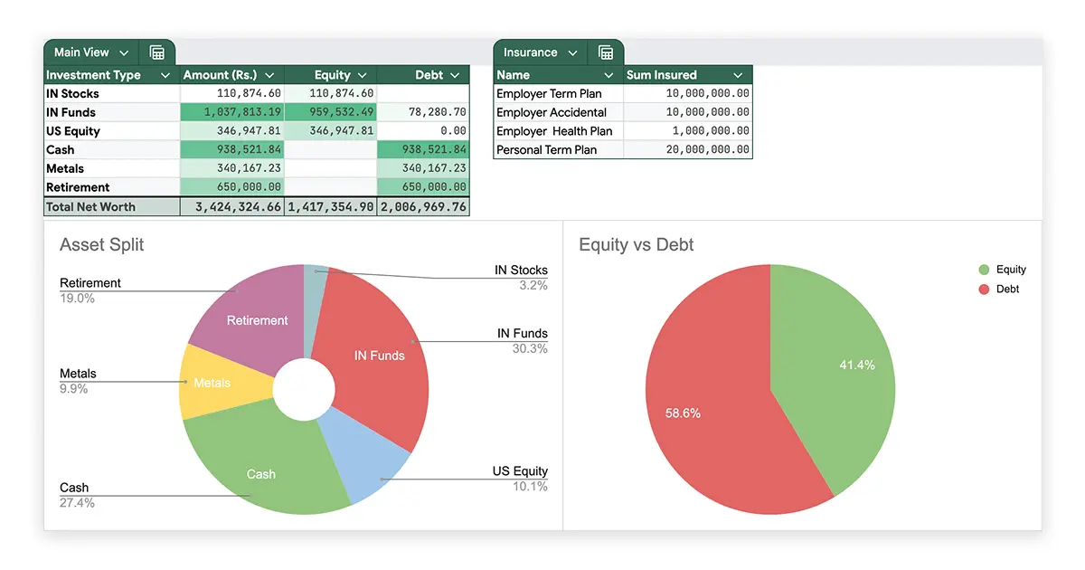
Net Worth Sheet
It contains the following tables and visualizations
| Name | What it tracks | Column |
|---|---|---|
| Main View | Indian Stocks and Funds, US Equity, Cash, Metals, Retirement | A |
| Insurance | Overview of Sum Insured against different types | B |
| Pie Chart #1 | Shows the asset split | C |
| Pie Chart #2 | Shows Equity vs Debt Split | D |
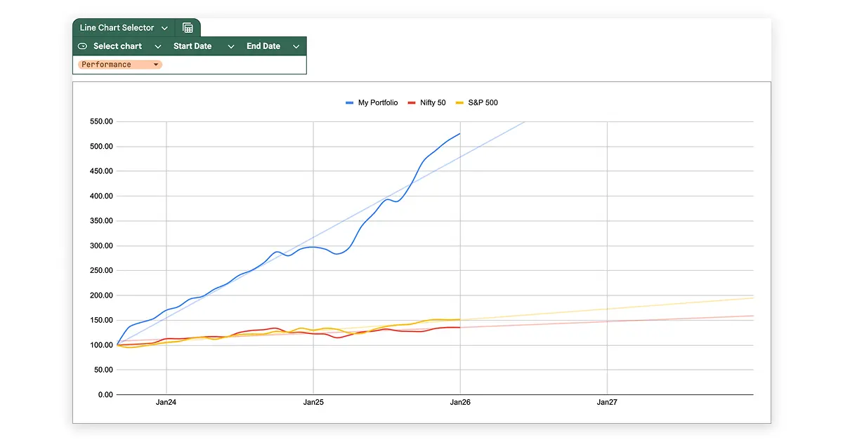
| Dynamic Line Chart | Can show 3 different line charts - 1. Total Net Worth, 2. Asset Trends, 3. Performance. These are toggled with a table named Line Chart Selector | E |
| Line Chart Selector | Table with a toggle to choose which line chart to view and two different cells to choose the time range for these charts. | F |
Monthly Tracker Sheet
It contains one table called the “Monthly Tracker” which has the following columns
| Name | What it tracks | Column |
|---|---|---|
| M/Y | The last date of each month | A |
| IN Stocks | Total value of Indian Stocks | B |
| IN Funds | Total value of Indian Funds | C |
| US Equity | Total value of US Equity | D |
| Cash | Total value of Cash and FD | E |
| Retirement | Total value of EPF and PPF | F |
| Metals | Total value of SGB, Gold and Silver | G |
| Net Worth | Total of all the assets of preceeding columns | H |
| Nifty50 & SP500 | Closing price of the index as of the date from the M/Y column of the same row | I |
| Portfolio | Total of IN Stocks,Funds,US Equity, Metals of the same row | J |
| Normalized Portfolio, N50 & SP500 | Normalized value of N50, SP500 and Portfolio column values of the same row | K |
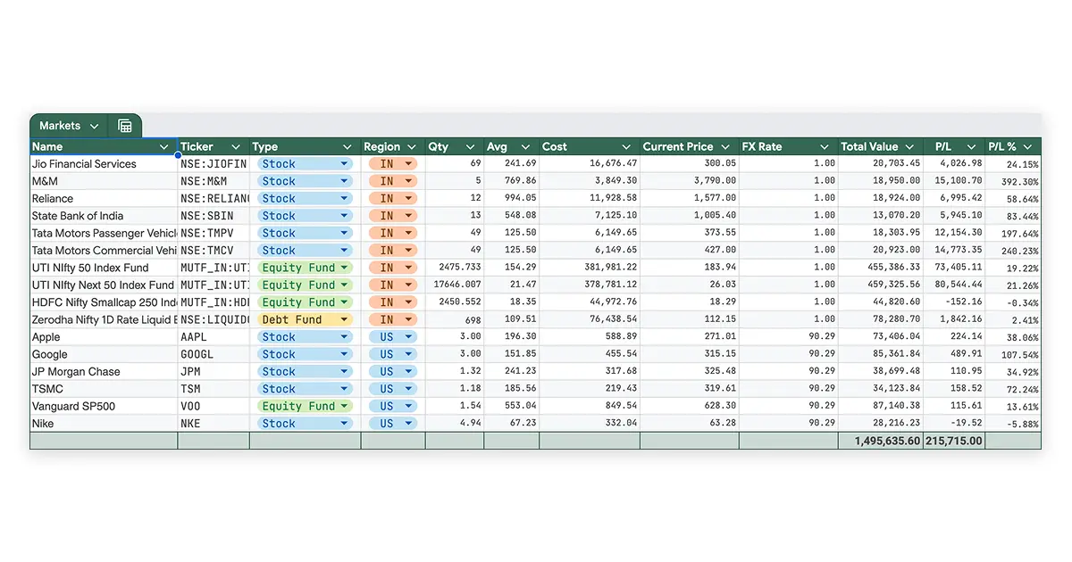
Markets Sheet
It contains one table called the “Markets” which has the following columns
| Name | What it tracks | Column |
|---|---|---|
| Name | Name of the stock/equity or debt fund | A |
| Ticker | Symbol of the stock/equity or debt fund | B |
| Type | Dropdown of stock/equity or debt fund | C |
| Region | Dropdown of IN or US | D |
| Qty | Number of stocks or units | E |
| Avg | Average price of a holding | F |
| Cost | Total invested amount of a holding | G |
| Current Price | Current price of a holding | H |
| FX Rate | Either 1 or the current USD-INR value. Used to multiply with the price to find the total current value of a holding in INR | I |
| Total Value | Total current value of a holding in INR | J |
| P/L | Total profit or loss of a holding | K |
| P/L% | Total profit or loss percentage of a holding | L |
Cash Sheet
It contains one table called the “Savings” which has the following columns
| Name | What it tracks | Column |
|---|---|---|
| Name | Description of the entry (eg: Cash/Salary ac etc) | A |
| Org | Bank/Broker etc | B |
| Type | Type of holding | C |
| Principal | Starting value of the holding | D |
| Start | Starting date for Fixed Depoits | E |
| End | Maturity date for Fixed Depoits | F |
| Interest | Interest for Fixed Deposits | G |
| Current Value | Current Value (as of today), same as Principal if Cash, Calculated if FD | H |
| Account # | Account numbers for holding | I |
Metals Sheet
It contains one table called the “Metals” which has the following columns
| Name | What it tracks | Column |
|---|---|---|
| Name | Name of the entry | A |
| Type | Dropdown of SGB/Gold/Silver | B |
| Cost @1 gram | Cost per gram during purchase | C |
| Grams | Total grams held | D |
| Making | Making charges for physical gold/silver | E |
| Total Cost | Total spending on a holding | F |
| Current Rate | Current rates pulled of a holding per gram | G |
| Total Value | Total value of a holding | H |
Retirement Sheet
It contains one table called the “Retirement” which has the following columns
| Name | What it tracks | Column |
|---|---|---|
| Name | Names of employers/bank etc | A |
| Type | EPF/PPF etc | B |
| Account # | Account numbers for holding | C |
| Total Value | Total Balance of the holding | D |
Insurance Sheet
It contains one table called the “Insurance Details” which has the following columns
| Name | What it tracks | Column |
|---|---|---|
| Insurance Company | Insurer’s name | A |
| Type | Dropdown of Term/Health/Accidental insurance | B |
| Policy # | Account number of the policy | C |
| Sum Insured | Total insured amount from the policy | D |
| Start Date | Start date of the policy | E |
| End Date | Maturity date of the policy | F |
Technical Logic
Named Ranges
Instead of manual ranges like A2:A9 or B2:B which could get complicated quickly as we scale the file based on various requirements, it gets incredibly important to use Named Ranges as they add labels to these ranges which are easier to reference. Also, once set up, these named ranges dynamically update whenever we add to or remove rows from these ranges.
For example: Using Markets_TotalValue is easier and easy to understand and reference rather than =Markets!J2:J40
Formulas
Many calculations and price detections are done using formulas. Currency conversions, Stocks, Mutual Funds and ETFs are directly supported by Google Sheets with the =googlefinance
function while prices of Gold, Silver, Platinum are auto fetched via the =importxml function.
On the Net Worth Sheet, the Main View table shows total current values of many assets. And as a lot of different assets tend to be in a single table, there are formulas that can filter and output the sum of only a particular type of asset.
For example, to only find the SUM of all the IN stocks from Markets sheet, here is the formula used in the B2 cell:
=IFERROR(
  SUM(
    FILTER(
      Markets_TotalValue,
      Markets_Region="IN",
      (Markets_Type="Stock")
    )
  ),
  0
)
Here,
Markets_Region&Markets_TotalValueare named ranges.
Here, IFERROR is a failsafe to return 0 if no value returned from the formula. FILTER used range and one of more conditions. SUM just sums up the all the values from the filtered range thus resulting in one Total value.
Similarly, you could also use this formula to return total of not just but multiple assets.
For example:
=IFERROR(
  SUM(
    FILTER(
      Markets_TotalValue,
      Markets_Region="US",
      (Markets_Type="Stock")
      + (Markets_Type="Equity Fund")
      + (Markets_Type="Debt Fund")
    )
  ),
  0
)
There are many other formulas throughout the sheet to calculate various things like Current Value of a Fixed Deposit etc.
To see all the formulas, refer the Glossary section.
Helper Sheet
The Helper Sheet which is hidden and protected (click on the All Sheets button to view) has a dynamic table ranging from cell A to E. This table enables the sheet to create different charts based on specific conditions.
As I wanted visualizations for Net worth trend, Asset Value Trend, Portfolio performance over time, Line charts seemed appropriate. However, I did not want to extend the vertical length of the page and thus a toggle to change charts in the same place seemed like the best idea.
There is a Line Chart Selector located below the pie charts with a dropdown toggle for Total Net Worth/Asset Trends/Performance and Start/End Date options to see these different line charts based on whatever time range the user wants.
These drop-down toggles trigger the formulas on the Helper sheet to change the table that shows up and the line chart uses this table to show the data.
This sheet should not be edited as it could break the visualizations or price fetching across the sheets.
There are two other tables on this sheet named Global Rates and Imported Rates per gm from column H.
The Global Rates table uses =GOOGLEFINANCE("CURRENCY:USDINR") to fetch the price of 1 USD in INR which is then used in the Markets sheet to convert the stock prices of holdings from the United States’ markets. This lets us use one single currency and thus discover the true value in Indian Rupee for consistency.
The Imported Rates per gm table on the other hand uses a somewhat unreliable source of price fetching. I used the IMPORTXML function to pull the daily price of gold silver and platinum from https://www.goodreturns.in/ website. It has different paths like /gold-rates/hyderabad.html, /silver-rates/hyderabad.html and /platinum-rate-in-hyderabad.html and these display the prices of said metals in a certain city on a static webpage. From there, I used the XPath of that particular amount on the page to be fetched on our helper cell.
For example, this is how the current gold price is fetched on I7 of the Helper sheet:
=importxml("https://www.goodreturns.in/gold-rates/hyderabad.html", "/html/body/div[1]/div[2]/div[1]/setion/div/div[1]/div[2]/p/span")
After this, we clean the extracted text using the following formula to normalize it to a number:
=Value((REGEXREPLACE(I7, "[₹,]", "")))
This is an unreliable way of fetching data. as it could break any time due to reasons like the website and its content being updated, it is important that we monitor the sheet for any inconsistency and if the fetching breaks, manually update the values in the helper sheet.
How to use
I like to track my portfolio once on the last day of each month. This reduced unnecessary anxiety and keeps the database clean for my taste. You will notice the same in the M/Y column of the Monthly Tracker sheet. It also allows me to see a Month-on-Month movement of my portfolio on the Line Charts.
You could essentially track Week-on-Week or even day to day movements but that would mean that your sheet would become enormous over time and may lag as well.
Tracking monthly means we have 12 rows in the Monthly Tracker sheet, while weekly means over 52 rows and 365 rows for daily tracking!
If you are content with my method, the first thing to do is to update the Insurance sheet and then in reversing order, we fill up all the remaining sheets up to the Markets sheet.
- For Insurance, we just add the description, select the type and add the sum insured and Start/End dates in the relevant fields. You may add the Policy numbers if you want to keep that handy.
- For Retirement, we add the Names, select the type and add the current balance in the relevant fields. You may add the Policy numbers if you want to keep that handy.
- For Metals, we add the Names and select the type of Metal. In “Cost @1gm”, we add the price we paid per gram for that metal type. In “Grams”, we add the total grams held. In “Making”, we add any relevant making charges. “Total Cost” calculates the total price paid for that metal. “Current rate” automatically fetches the current price of that metal. “Total Value” calculates the total current value.
The “Current Rate” for SGBs need to be manually entered.
- For Cash, we add the Names, Orgs and select the type. In “Principal”, we add the initial invested amount (For Cash type, this would be the current balance). In “Start” and “End” fields, we enter the starting and maturity dates for FD type only. In “Interest”, we enter the percentage of interest offered for that FD. The “Current Value” calculates the total current value of that FD and just duplicates the balance(principal) amount for cash type. “Account #” can be used to store account numbers.
- For Markets, we add the Names, Tickers (pulled from Google Finance) and select the type of asset and region. In “Qty” we enter the number of Stocks or Units held. In “Cost” we enter the total invested amount for that asset. The “Avg” field auto-calculates the average price for a particular asset by dividing Cost by Quantity. “Current Price” fetches the current price of that asset. “FX Rate” shows 1 for Indian assets and the current USD to INR rate for US assets. “Total Value” calculates the Total Current value of that holding by multiplying Quantity, Current Price and FX rate. “P/L” and “P/L %” calculates the profit and loss of that holding in absolute and percentage.
After we have filled all these sheets, the Main View table on the Net Worth Sheet should have auto populated the total values for all asset and debt types. We can now also see our Total Net Worth, Pie charts showing Equity vs Debt split and Asset type split.
From here, we can copy the total values of each asset/debt types, once every month into the relevant fields of Monthly Tracker sheet. This will then enable the three interchangeable Line Charts in the main sheet.
The line charts will need a few rows in Monthly tracker to correctly show the growth/fall and trend lines.
If you find any issues with this tool or would like to discuss it further, feel free to reach out at me@harshnahar.com
Glossary of formulas
Simple formulas like “=G2 + B2” or “=B2” are not mentioned in this list.
| Syntax | Location | Purpose | |
|---|---|---|---|
| 1 | =IF('Net Worth'!$A$29="Total Net Worth", "Net Worth", IF('Net Worth'!$A$29="Asset Trends", "Indian Stocks", "My Portfolio")) |
Helper - B2 | Name the cell a specific word based on a condition that checks other sheets |
| 2 | IF('Net Worth'!$A$29="Total Net Worth", "", IF('Net Worth'!$A$29="Asset Trends", "Indian MF", "Nifty 50")) |
Helper - C2 | Name the cell a specific word based on a condition that checks other sheets |
| 3 | =IF('Net Worth'!$A$29="Total Net Worth", "", IF('Net Worth'!$A$29="Asset Trends", "US Equity", "S&P 500")) |
Helper - D2 | Name the cell a specific word based on a condition that checks other sheets |
| 4 | =IF('Net Worth'!$A$29="Asset Trends", "Metals", "") |
Helper - E2 | Name the cell a specific word based on a condition that checks other sheets |
| 5 | =FILTER('Monthly Tracker'!A2:A, 'Monthly Tracker'!A2:A >= IF('Net Worth'!$B$29="", 0, 'Net Worth'!$B$29),'Monthly Tracker'!A2:A <= IF('Net Worth'!$C$29="", 99999, 'Net Worth'!$C$29)) |
Helper - A3 | Copy all the dates from Monthly tracker sheet in one column. If the Line Chart Selector has a date range, only copy the dates within the date range |
| 6 | =GOOGLEFINANCE("CURRENCY:USDINR") |
Helper - Global Rates - I2 | Fetch the live USD to INR value |
| 7 | =importxml("https://www.goodreturns.in/gold-rates/hyderabad.html", "/html/body/div[1]/div[2]/div[1]/setion/div/div[1]/div[2]/p/span") |
Helper - Global Rates - I7 | Import the live 24k gold value from goodreturns.in |
| 8 | =importxml("https://www.goodreturns.in/gold-rates/hyderabad.html", "/html/body/div[1]/div[2]/div[1]/setion/div/div[2]/div[2]/p/span") |
Helper - Global Rates - I8 | Import the live 22k gold value from goodreturns.in |
| 9 | =importxml("https://www.goodreturns.in/silver-rates/hyderabad.html", "/html/body/div[1]/div[2]/div[1]/section[3]/div/div[1]/div[2]/p/span") |
Helper - Global Rates - I9 | Import the live silver value from goodreturns.in |
| 10 | =importxml("https://www.goodreturns.in/platinum-rate-in-hyderabad.html", "/html/body/div[1]/div[2]/div[1]/section[3]/div/div[1]/div[2]/p/span") |
Helper - Global Rates - I10 | Import the live platinum value from goodreturns.in |
| 11 | =Value((REGEXREPLACE(I7, "[₹,]", ""))) |
Helper - Global Rates - J7 | Trim unnecessary characters from imported values in I7 and Normalize the value to a number |
| 12 | =Value((REGEXREPLACE(I8, "[₹,]", ""))) |
Helper - Global Rates - J8 | Trim unnecessary characters from imported values in I8 and Normalize the value to a number |
| 13 | =Value((REGEXREPLACE(I9, "[₹,]", ""))) |
Helper - Global Rates - J9 | Trim unnecessary characters from imported values in I9 and Normalize the value to a number |
| 14 | =Value((REGEXREPLACE(I10, "[₹,]", ""))) |
Helper - Global Rates - J10 | Trim unnecessary characters from imported values in I10 and Normalize the value to a number |
| 15 | =IFERROR(SUM(FILTER(Markets_TotalValue,Markets_Region="IN", (Markets_Type="Stock"))),0) |
Net Worth - Main View - B2 | Filter the Markets_TotalValue range based on the IN and Stock categories and return the total value |
| 16 | =IFERROR(SUM(FILTER(Markets_TotalValue,Markets_Region="IN", (Markets_Type="Equity Fund")+(Markets_Type="Debt Fund"))),0) |
Net Worth - Main View - B3 | Filter the Markets_TotalValue range based on the IN and Equity Fund, Debt Fund categories and return the total value |
| 17 | =IFERROR(SUM(FILTER(Markets_TotalValue,Markets_Region="IN",(Markets_Type="Equity Fund"))),0) |
Net Worth - Main View - C3 | Filter the Markets_TotalValue range based on the IN and Equity Fund categories and return the total value |
| 18 | =IFERROR(SUM(FILTER(Markets_TotalValue,Markets_Region="IN",(Markets_Type="Debt Fund"))),0) |
Net Worth - Main View - D3 | Filter the Markets_TotalValue range based on the IN and Debt Fund categories and return the total value |
| 19 | =IFERROR(SUM(FILTER(Markets_TotalValue,Markets_Region="US",(Markets_Type="Stock")+(Markets_Type="Equity Fund")+(Markets_Type="Debt Fund"))),0) |
Net Worth - Main View - B4 | Filter the Markets_TotalValue range based on the US and Stocks, Equity Fund, Debt Fund categories and return the total value |
| 20 | =IFERROR(SUM(FILTER(Markets_TotalValue,Markets_Region="US",(Markets_Type="Stock")+(Markets_Type="Equity Fund")))),0) |
Net Worth - Main View - C4 | Filter the Markets_TotalValue range based on the US and Stocks, Equity Fund categories and return the total value |
| 21 | =IFERROR(SUM(FILTER(Markets_TotalValue,Markets_Region="US",(Markets_Type="Debt Fund"))),0) |
Net Worth - Main View - D4 | Filter the Markets_TotalValue range based on the US and Debt Fund categories and return the total value |
| 22 | =IFERROR(SUM(FILTER(Cash_TotalValue,(Cash_Type = "Cash")+(Cash_Type = "FD"))),0) |
Net Worth - Main View - B5 | Filter the Cash_TotalValue range based on the Cash and FD categories and return the total value |
| 23 | =IFERROR(SUM( FILTER(Metals_TotalValue,(Metals_Type="SGB") + (Metals_Type="Gold") + (Metals_Type="Silver"))), 0) |
Net Worth - Main View - B6 | Filter the Metals_TotalValue range based on the SGB, Gold, Silver categories and return the total value |
| 24 | =IFERROR(SUM(FILTER(Retirement_TotalValue,(Retirement_Type="EPF")+(Retirement_Type="PPF")+(Retirement_Type="Leave"))),0) |
Net Worth - Main View - B7 | Filter the Retirement_TotalValue range based on the EPF, PPF categories and return the total value |
| 25 | =INDEX(GOOGLEFINANCE("INDEXNSE:NIFTY_50", "close",A2),2,2) |
Monthly Tracker - Monthly Tracker - I2 | Fetch the Closing Price of Nifty 50 Index for the date mentioned in the same row |
| 26 | =INDEX(GOOGLEFINANCE("INDEXSP:.INX", "close", A2),2,2) |
Monthly Tracker - Monthly Tracker - J2 | Fetch the Closing Price of S&P 500 Index for the date mentioned in the same row |
| 27 | =(I2 / $I$2) * 100 |
Monthly Tracker - Monthly Tracker - K2 | Normalize the values from Nifty 50 Index closing price, starting from 100 |
| 28 | =(J2/$J$2) * 100 |
Monthly Tracker - Monthly Tracker - L2 | Normalize the values from S&P 500 Index closing price, starting from 100 |
| 29 | =(M2/$M$2) * 100 |
Monthly Tracker - Monthly Tracker - N2 | Normalize the values from our investment portfolio in the Portfolio column, starting from 100 |
| 30 | =GOOGLEFINANCE(insert the Ticker symbol cell of the corresponding row ) |
Markets - Markets - Current Price Column | Fetch the current price of the corresponding holding |
| 31 | =IF(D2="US", Helper!$I$2, 1) |
Markets - Markets - FX RateColumn | Return 1 if “IN” or the USD-INR rate “US” if is selected in the region column |
| 32 | =IFERROR(SWITCH(C7,"Cash",D7, "FD",IF(G7=0,D7,D7 * (1 + G7/100) ^ (DATEDIF(E7, MIN(TODAY(), F7), "D") / 365),0),0) |
Cash - Savings - Current Value Column | Return the same principal value if “Cash” and the current FD Value if FD is selected in the type column |